II. Cost-Distance Analysis

Most cartographic distance calculations are performed in coordinate systems such as the metric Universal Transverse Mercator (UTM) where space is evenly divided into equal-sized units. In practice, however, people often conceive of distances in terms of time or effort. In mountainous settings the isotropic assumptions of metric map-distance calculations are particularly misleading because altitude gained and lost, and other obstacles such as cliff faces, are typically not factored into the travel estimate. Cost-distance functions are a means of representing such distances in terms of units of time or caloric effort.

In this exercise we will use an algorithm, one based primarily on slope from a topographic surface, to derive both an optimal route across that surface (Least-cost Path) as well as estimated time to cross that surface. Please see the ESRI manual on Path-distance and for a more thorough explanation see the general Cost-distance explanation as well. Here we are performing a pathdistance calculation using a customized cost function that reflects empirical data published by Tobler, 1993. Tobler's function estimates time (hours) to cross a raster cell based on slope (degrees) as calculated on a DEM.

I have converted data provided by Tobler into a structure that ArcGIS will accept as a "Vertical Factor Table" for the Path Distance function. In other words, ArcGIS makes these sorts of calculations easy by allowing you to enter customized factors to the cost function.

  A. ISOTROPIC TIME ESTIMATE

1. Distance and time estimates based on 4 km/hr speed on an isotropic surface

This exercise begins by calculating distance and estimating time done in the old fashioned way, assuming a flat surface, as you would do on a map with a ruler.

We will begin by creating an isotropic cost surface and then generating 15 min isolines on this surface.

• Download the file [ViewCost.zip] and load the files into Arcmap.

• Open the attribute table for Sites and choose the row with the value ArchID = 675.

Hint: Sort Ascending ArchID column, and hold down ctrl button while you click the left-most column in the table for those two rows.

• Go to Toolbox > Spatial Analyst Tools > Distance > Euclidean Distance [Make sure Spatial Analyst extension is turned on under Tools > Extensions]

Input Feature: Sites
Output Dist Raster: EucDist_Site1
[click folder and save it in the same DEM folder]
Output cell size: 30
Leave the other fields blank.

• Before clicking OK click the Environments… button at the bottom of the window.

• Click the General Settings… tab and look at the different settings. Change the Output Extent field (General Settings) to read "Same as layer colca_aster".

2. Create raster showing isotropic distance in minutes

The output is a raster showing the metric distance from the site.
Let's assume for the purposes of this example that hiking speed is 4 km/hr regardless of the terrain, which works out to 1000m each 15 min.

• To transform the EucDist_Site1 grid into units of time (minutes) we can perform a Spatial Analyst menu > Raster Calculator expression using this information:
  15 min / 1000 meters = 1 min / 66.66 meters

To construct that equation in Raster Calculator to get the raster to display in units of minutes we would divide the distance raster by 66.66. Built up the equation like so:

Double click EucDist_Site1 layer, click / button, then type in 66.66

If you've done it right the output raster (Calculation) will range in value from
0 to 204.897

• When you have this raster right click and choose "Make Permanent…", and call it "isodist_min". Remove the Calculation grid layer and add this "isodist_min" grid to your project.

3. Convert to isochrones

• Create contours using the output raster with
  Spatial Analyst toolbar > Surface Analysis > Contour…

• Then use the good Calculation raster as your input surface, choose 15 as your interval and use the defaults for the rest. Save the file out as "isochrone15" (click the folder to specify the target directory).

What do you think of the results of these lines?

The photo at the top of this webpage was taken facing south towards Taukamayo which lies in the background on the right side of the creek in the center-left of the photo. Taukamayo is the western-most of the two sites you just worked with in Arcmap. You can see how steep the hills are behind the site and on the left side of the photo you can see the town of Callalli for scale. Clearly the land is very steep around the site, especially in those cliff bands on the south end of the DEM. There are also cliffbands on the north side of the river but the river terrace in the foreground where the archaeologists are standing is quite flat.

 B. ANISOTROPIC TIME ESTIMATE USING PATH DISTANCE

 1. An algorithm is needed to convert from Slope to Time

In ArcGIS the PathDistance function can be used to conduct anisotropic distance calculations if we supply the function with a customized Vertical Factor table with the degree slope in Column 1 and the appropriate vertical factor in Column 2. The vertical factor acts as a multiplier, and multiplying by a Vertical Factor of 1 has no effect. The vertical factor table we will use was generated in Excel and it reflects Tobler's Hiking Function by using the reciprocal of Tobler's function. This function was used in Excel:

TIME (HOURS) TO CROSS 1 METER or the reciprocal of Meters per Hour =0.000166666*(EXP(3.5*(ABS(TAN(RADIANS(slope_deg))+0.05))))

Thus for 0 deg slope which Tobler's function computes to 5.037km/hr, the result should be 1/5037.8 = 0.000198541

You can download the file that we will use for these values here.

Right-click ToblerAway.txt, choose"Save Link as..." and save it in the same folder as your GRID files (the reciprocal ToblerTowards.txt is used for travel in the opposite dirction, towards the source).

An abbreviated version of this ToblerAway file looks like this 

  2. Pathdistance Calculation

Once again select from the Sites attribute table the locations with ARCHID values of  675.

Type 80,000 in the scale field at the top toolbar and position the selected site in roughly the middle of the window

Go to ArcToolbox > Spatial Analyst Tools > Distance > Path Distance...

• Input: Sites
• Output: aniso_hrs1  [click the folder and navigate to (on these computers) the directory called D:\arch_workshop2009\ so the Path should read: D:\arch_workshop_2009\aniso_hrs1 ]
• Input cost:<blank>
• Input surface: colca_aster (our 30m DEM)
• Output Backlink raster: aniso1_bklk [put it in D:\arch_workshop_2009\ ]

• Open the "Vertical factor parameters" field
• Input Vertical Raster: colca_aster
• Vertical Factor: Table (scroll down to bottom of menu list)
• browse to find "Tobler_away.txt" on your hard drive

One more thing:

• Click "Environments..." at the bottom of the window
• Open "General Settings..."
• Set the Extent to "Same as Display"

You may get a geoprocessing engine error ... if so, remove this last step setting the Extent.

3. Inspect your results carefully and convert units if necessary

Turn off the aniso1_bklk file so that you're viewing aniso1_hrs. 

Why aren't the values larger? Recall what units the Tobler_Away function calculates?

We need to multiply this result by 60 because…. It's in hours.

• Spatial Analyst toolbar > Raster Calculator…
  [aniso1_hrs] * 60   ( note that you must have spaces between the variables and the operators in Raster Calculator.When in doubt, add a space )
• Right-click the Output Calculation and Make Permanent… Call it "aniso1_min" and save it into D:\arch_workshop_2009\

• Now generate 15 min contours on this layer as you did earlier and call the output "aniso15".
• Turn off all layers except Callalli_DEM", "Hydro", "isochrone15" and "aniso15".
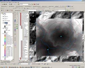
• Do you see the difference in the two cost surfaces?

In this image the black circles are Isochrones incrementing by 15 minutes, while the background raster shows the Anisotropic distance calculation with red lines showing 15 min increments away from the site.

Using the Info tool (the blue 'i') you can point-sample distances along the way against the layer aniso1_min and isodist_min.

The differences between the two surfaces can be interesting

• Spatial Analyst > Raster Calculator...
• [aniso_min] - [isodist_min]

Symbolize the output raster using a Red to Blue gradient fill and look at the result. What are the high and low values showing?

PART C. GENERATING LEAST-COST PATHS BETWEEN SITES

Recall that you generated a Backlink grid called aniso1_bklk as part of the PathDistance calculation. We will now use that to calculate least-cost paths between the two sites and other sites in the region. 

First, we need to generate a 

• Add Backlink Grid to Arcmap called "aniso1_bklk".

Look at the results. Recall how Backlink Grids work (read about the Direction raster in the Help on Cost Distances), do the values 0 through 8 make sense?

Choose three sites from ArchID for this calculation
607, 611, 811, 837, 926

• Let's construct this selection in ArchID from the Attribute Table using Options button > Select by Attributes…

It should look something like this
[ARCHID] = 607 OR [ARCHID] =611 OR [ARCHID] = 811 OR [ARCHID] = 837 OR [ARCHID] = 926

• Now close the attribute table. You have four sites selected around the perimeter of the study area?

• Choose Toolbox > Spatial Analyst Tools > Distance > Cost Path…

Input Feature: Sites
Destination Field: ArchID
Input Cost Distance Raster: aniso_hours (use the hours not the minutes one)
Input Cost Backlink Raster: aniso_bklk

Note that the output is a raster GRID file. Wouldn't these be more useful as Polylines?

• Use Spatial Analyst > Convert > Raster to feature….

Input Raster: <the name of your cost paths file>
Field: Value
Geometry type: Polyline

Zoom in and explore the results with only the following layers visible:

Callalli_DEM, Hydro_lines100k, aniso_minutes isolines, and the cost-paths you just generated. Note how the paths avoid steep hills and choose to follow valleys, as you might do if you were planning to walk that distance.