I. Viewshed Analysis 2009
This exercise will demonstrate two types of viewshed analysis.The first is a single site Viewshed, and the second is a general measure of visibility or exposure.
To begin with, please download and unzip the following dataset: 2009_View_Cost.zip (2mb).
Place the data in a directory under C:\ (not in My Documents) so that the path is simple and has no spaces. You might use
C:\gis_data\
Note: these data are derived from my dissertation data but the attributes have been altered for this workshop.
1. Setup the project in Arcmap.
- Add the Sites shapefile.
- Add the Hydro_lines100k Shapefile.
- Add the 30m ASTER DEM from \dem\
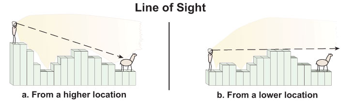
Look at the coordinates in the lower right corner. Is this in UTM or in Decimal Degrees? With Viewshed analysis linear units (like Meters) are necessary to accurately calculate distances.For more information on projected and unprojected data in GIS see the ESRI Coordinate Systems help and Peter Dana's online tutorials.
Look at the Attribute table for Sites. I won't explain the attributes here (see other labs in the GIS and Anthropology course) but the ARCHID field is a unique ID field for each feature in this Shapefile.
We'll use the "Period" field to differentiate sites from different time periods in this study.
The values are
- Formative (2000BC - AD400)
- MH Middle Horizon (AD400-AD1100), there are no MH sites in this dataset
- LIP Late Intermediate Period: (AD1100-AD1476)
- LH Late Horizon (AD1476-AD1532)
Note that the last attribute "View_Code" is a numerical representation of the Period field.
2. How do we control the viewshed calculation?
Please see the explanation on this webpage: ArcGIS Help - Viewshed
The optional viewshed parameters are SPOT, OFFSETA, OFFSETB, AZIMUTH1, AZIMUTH2, VERT1, and VERT2. These attribute fields will be used by the Viewshed function if they are present in the feature observer (Sites) attribute table.


The only two attribute variables we are concerned with at this point are OFFSETA (height of viewer) and RADIUS2 (the maximum radius of the viewshed calculation).
The viewer's eyes are at 1.5m above the ground, and we want to know the visible area within 5 km of each site.
In order to setup the analysis we need to add these values to fields in the Sites attribute table.
- Make sure nothing is selected in Arcmap [Selection menu > Clear Selected Features].
- Open the Attribute Table for the Sites layer [Right click Sites layer > Open Attribute Table].
- Choose Options (at bottom of table) > Add Field…
- Call it OFFSETA, make the type FLOAT and the Precision 2 and the scale 1.
Precision sets the number of significant digits, while the Scale is the location of the decimal point from the right side of the value. These settings allow the field to store "1.5".

- Use Calculate Values... command to put 1.5 in the field for the whole table. [Right-click field header OFFSETA > Field Calculator
- Choose Add field... again
- Call it RADIUS2 and leave it as the default: Short Integer
Question: Since we want to limit the value of the view to 5 km, what should the value be in that goes in this field? What are the spatial units of this map in the UTM coordinate sys?
Answer:You can use Calculate Values... command to fill the RADIUS2 field with the value 5000 (meters) all the way down.
3. A quick viewshed analysis
For the next step you need to make sure your Spatial Analyst extension is turned on [Tools > Extensions > Spatial Analyst] and that the Spatial Analyst toolbar is visible [View > Toolbars > Spatial Analyst]
- Make sure nothing is selected in Arcmap.
- go to Spatial Analyst toolbar > Surface Analysis > Viewshed…
Input: Colca_Aster
Observer Points: Sites
Use the defaults [Z=1, Size=30m] and allow the output to go into Temporary.
Look at the result. What is this showing? Is this informative?
Put the Colca_HS (hillshade) layer above the Viewshed output at 60% transparency:
- Drag Colca_HS above the Viewshed layer in the Layers list.
- Right click Colca_HS and click Display tab.
- Enter 60 in Transparency field.
This help you to visualize what is happening. Note that none of the Sites are within 5 km of the border of the DEM so there are no "Edge Effects" from the analysis running off of the edge of the DEM.
4. Viewshed analysis - differences between time periods
What is missing from the previous analysis was a theoretical question guiding the inquiry. Obviously, you can select a single site and run a viewshed and find out the resulting area. But how is this different from just going to the site and looking around and taking photos?
You could also select a line and find the viewshed along a road, for example. However, GIS has made it easier to pursue interesting questions by looking at general patterns with larger datasets. This is where computers give you an advantage because you're repeating many small operations.
We want to answer questions such as:
- How do viewsheds change based on the type of site that is being evaluated?
- Are Late Intermediate sites more or less likely to be constructed such that they can view one another?
We can calculate separate viewsheds for each group of sites in our table by manually selecting each group from the Attribute Table and running the viewshed calc. Exploring viewsheds for different subsets of the Sites file is a good application of the ModelBuilder feature in ArcGIS, however we won't be using it in this workshop (see this Yale Library GIS workshop for a Model Builder viewshed tutorial).
1. Calculate viewshed for each major group:
We will manually select groups of Sites by Attribute and compare the viewsheds between them.
- Open the Sites Attribute table, Sort Ascending on the "Period" field.
- Select only the Formative sites
- Use Spatial Analyst > Surface Analysis > Viewshed…
- This time change the "Output Raster:" field to be "Form5km" and save it to the viewshed folder.
- MAKE SURE the INPUT SURFACE IS COLCA_ASTER (it will default to the wrong GRID file!).
- Repeat the above process two more times with LH and LIP, calling the output GRID files LH5km and LIP5km respectively. Turn these three layers on and off and investigate their respective Visible areas.

5. Consider the implications of your results carefully and bring them to other software.
The results of viewshed analysis are a bit of a puzzle to think through. Consider the issue of intervisibility: are you assuming that everyone who is "in view" can in turn percieve their viewer? What about camouflage, or hiding behind hilltops?
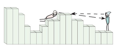 A non-reciprochal viewshed |
The size of the target, the target against a background, the air quality, and visual acuity of the viewer are all factors. Many such assumptions should be considered before deriving strong conclusions from these analyses.
Numerically, we can explore these results and you may want to bring the data out of ArcGIS for statistical analysis. First, have a look at the output GRID Attribute table for the Form5km GRID file. The VALUE field indicates how many of the sites can view a given cell, and the COUNT field indicates how many cells fall into that category.
In other words, in Form5km GRID the VALUE = 3 row shows that 1823 cells are visible from 3 sites and 88 cells are visible from all 4 formative sites.You can export these Attribute Table data to a comma-delimited Text file by going to the Options... button at the bottom of the window and choosing Options > Export... and Text format.
Analyses of Results
Alternately, instead of comparing between time periods you could use Site Type field designation to evaluate the viewsheds of "Pukaras" versus "Settlement" site types (for LIP sites only). Unsurprisingly, Pukara sites have much larger viewsheds.
Zonal Statistics
An important tool for analyzing geoprocessing results like Viewshed is the Zonal Statistics tool. Basically, this tool allows you to derive results from evaluating data in Vector form against data in Raster form. In this case, we can investigate patterning in viewsheds by time period such as "How many Formative sites fall in raster 'zones' visible from LIP sites (LIP viewsheds)? Contemporaneity issues aside, this allows us to look at settlement pattern changes.
Procedure:
Select all the Sites from the Formative using the Attribute Table values.
Spatial Analyst menu > Zonal Statistics...
Zone dataset: Sites
Zone field: ArchID
Value Raster: Viewshed of LIP sites
Check "Join output table to zone layer"
and put the Output table in your 2009 Workshop directory.
 The output from this analysis is a table with a row for each Formative site in your selection (so that the tables can be joined), and then with columns showing the values of the raster underneath those selected site locations. In this case, the values are mostly 0 which shows you numerically that despite the high viewsheds of the LIP, the Formative settlement patterns was quite different.
Zonal Histogram is a new tool to generate a frequency plot using the symbology of your Raster layer.
Other analyses:
We could calculate the number of cells in view per site, or other types of averages.
For example, in the Sites Attribute table there is a SiteType field that indicates that some of the LIP sites are Pukaras. These are hilltop defensive structures that have notoriously good views. We could determine the degree of intervisibility between LIP pukara sites numerically.
However… there's a problem. The problem lies in the bias in our sample because sites tend to aggregate around resource patches or other features. In these areas our dataset has high "intervisibility" because it reflects aggregation within the 5km buffer. In other words, many sites can see a particular cell in those situations where there are many sites in a small area!
We can get around this problem by calculating viewshed for random site locations as representative of "typical" views in the area. We will then compare our site views against this typical viewshed. This is called a Cumulative Viewshed Analysis and there isn't time to do that this workshop.
Viewshed - A few relevant references
Lake, Mark W., P. E. Woodman and Stephen J. Mithen
1998 Tailoring GIS software for archaeological applications: An example concerning viewshed analysis. Journal of Archaeological Science 25(1):27-38.
Llobera, Marcos
2003 Extending GIS-based visual analysis: the concept of visualscapes. International Journal of Geographical Information Science 17(1):25-48.
Ogburn, Dennis E.
2006 Assessing the level of visibility of cultural objects in past landscapes. Journal of Archaeological Science 33(3):405-413.
Tripcevich, Nicholas
2002 Viewshed Analysis of the Ilave River Valley. Master's Thesis.
Tschan, André P., Wldozimierz Raczkowski and Malgorzata Latalowa
2000 Perception and viewsheds: Are they mutually exclusive? In Beyond the map: Archaeology and spatial technologies, edited by G. R. Lock, pp. 28-48. IOS Press, Amsterdam.
Wheatley, David
1995 Cumulative Viewshed Analysis: a GIS-based method for investigating intervisibility and its archaeological application. In Archaeology and GIS: a European perspective, edited by G. Lock and Z. Stancic. Routlege, London.
Wheatley, David and Mark Gillings
2002 Spatial technology and archaeology: the archaeological applications of GIS. Taylor & Francis, London ; New York.